40 change data labels in excel chart

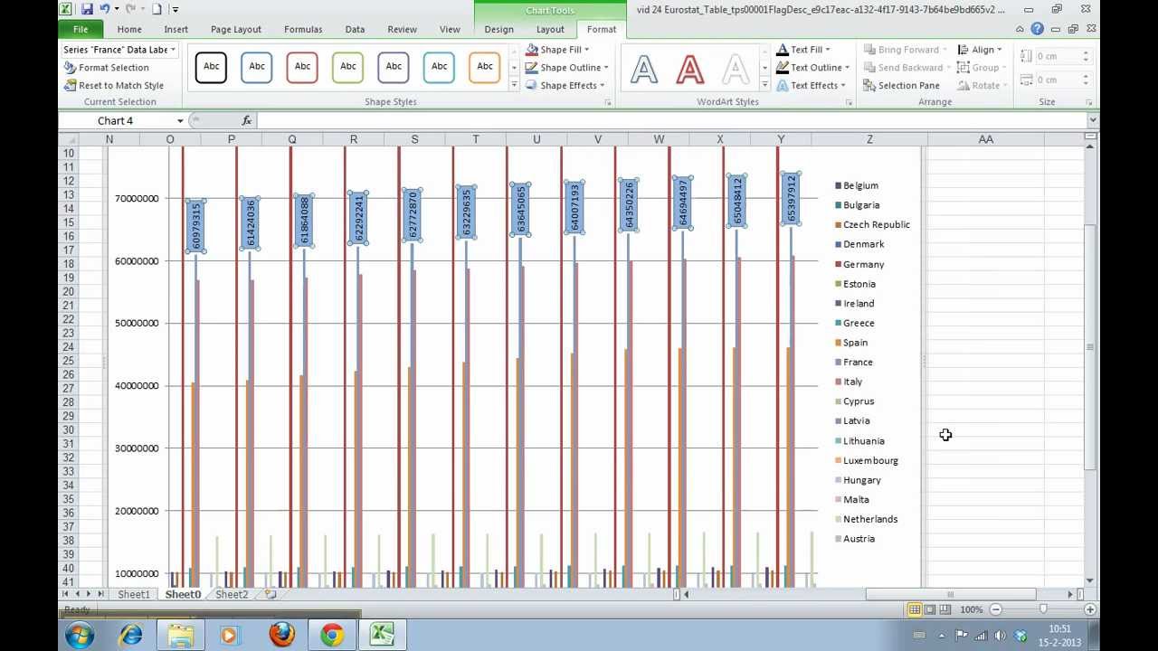
Change the format of data labels in a chart To get there, after adding your data labels, select the data label to format, and then click Chart Elements > Data Labels > More Options. To go to the appropriate area, click one of the four icons ( Fill & Line , Effects , Size & Properties ( Layout & Properties in Outlook or Word), or Label Options ) shown here. How to rotate axis labels in chart in Excel? - ExtendOffice 1. Go to the chart and right click its axis labels you will rotate, and select the Format Axis from the context menu. 2. In the Format Axis pane in the right, click the Size & Properties button, click the Text direction box, and specify one direction from the drop down list. See screen shot below:

How to add or move data labels in Excel chart? - ExtendOffice In Excel 2013 or 2016. 1. Click the chart to show the Chart Elements button . 2. Then click the Chart Elements, and check Data Labels, then you can click the arrow to choose an option about the data labels in the sub menu. See screenshot: In Excel 2010 or 2007. 1. click on the chart to show the Layout tab in the Chart Tools group. See ...

Change data labels in excel chart

Move data labels - support.microsoft.com Click any data label once to select all of them, or double-click a specific data label you want to move. Right-click the selection > Chart Elements > Data Labels arrow, and select the placement option you want. Different options are available for different chart types. Add or remove data labels in a chart - support.microsoft.com Click the data series or chart. To label one data point, after clicking the series, click that data point. In the upper right corner, next to the chart, click Add Chart Element > Data Labels. To change the location, click the arrow, and choose an option. If you want to show your data label inside a text bubble shape, click Data Callout. How to change Axis labels in Excel Chart - A Complete Guide Right-click the horizontal axis (X) in the chart you want to change. In the context menu that appears, click on Select Data…. A Select Data Source dialog opens. In the area under the Horizontal (Category) Axis Labels box, click the Edit command button. Enter the labels you want to use in the Axis label range box, separated by commas.

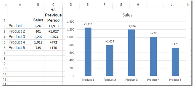
Change data labels in excel chart. How to create Custom Data Labels in Excel Charts - Efficiency 365 Create the chart as usual. Add default data labels. Click on each unwanted label (using slow double click) and delete it. Select each item where you want the custom label one at a time. Press F2 to move focus to the Formula editing box. Type the equal to sign. Now click on the cell which contains the appropriate label. How to add data labels from different column in an Excel chart? Right click the data series in the chart, and select Add Data Labels > Add Data Labels from the context menu to add data labels. 2. Click any data label to select all data labels, and then click the specified data label to select it only in the chart. 3. How to change axis labels order in a bar chart - Microsoft Excel 365 See more about the competition chart. To change the order of the labels on the axis, do the following: 1. Right-click the horizontal axis and click the Format Axis... in the popup menu (or double-click the axis): 2. On the Format Axis pane, on the Axis Options tab, in the Axis Options group: Under Axis position, select the Category in reverse ... How to change chart axis labels' font color and size in Excel? Sometimes, you may want to change labels' font color by positive/negative/0 in an axis in chart. You can get it done with conditional formatting easily as follows: 1. Right click the axis you will change labels by positive/negative/0, and select the Format Axis from right-clicking menu. 2. Do one of below processes based on your Microsoft Excel ...

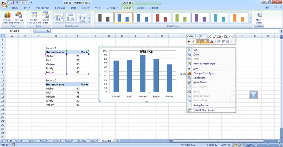
How to Edit Pie Chart in Excel (All Possible Modifications) How to Edit Pie Chart in Excel 1. Change Chart Color 2. Change Background Color 3. Change Font of Pie Chart 4. Change Chart Border 5. Resize Pie Chart 6. Change Chart Title Position 7. Change Data Labels Position 8. Show Percentage on Data Labels 9. Change Pie Chart's Legend Position 10. Edit Pie Chart Using Switch Row/Column Button 11. Change order of data labels in chart - Microsoft Community Replied on March 4, 2013. In reply to Ty_hell_heaven's post on March 4, 2013. The data were added in the order shown in the list before realizing that the labels could not be moved around. The order of the labels on the right should be, downward, 10, 8, 6, 4, and 2. Report abuse. Add / Move Data Labels in Charts - Excel & Google Sheets Adding Data Labels Click on the graph Select + Sign in the top right of the graph Check Data Labels Change Position of Data Labels Click on the arrow next to Data Labels to change the position of where the labels are in relation to the bar chart Final Graph with Data Labels How to Add Data Labels in Excel - Excelchat | Excelchat In Excel 2013 and the later versions we need to do the followings; Click anywhere in the chart area to display the Chart Elements button Figure 5. Chart Elements Button Click the Chart Elements button > Select the Data Labels, then click the Arrow to choose the data labels position. Figure 6. How to Add Data Labels in Excel 2013 Figure 7.

Custom Chart Data Labels In Excel With Formulas Follow the steps below to create the custom data labels. Select the chart label you want to change. In the formula-bar hit = (equals), select the cell reference containing your chart label's data. In this case, the first label is in cell E2. Finally, repeat for all your chart laebls. Data Labels in Excel Pivot Chart (Detailed Analysis) Next open Format Data Labels by pressing the More options in the Data Labels. Then on the side panel, click on the Value From Cells. Next, in the dialog box, Select D5:D11, and click OK. Right after clicking OK, you will notice that there are percentage signs showing on top of the columns. 4. Changing Appearance of Pivot Chart Labels How to Change Excel Chart Data Labels to Custom Values? May 05, 2010 · Now, click on any data label. This will select “all” data labels. Now click once again. At this point excel will select only one data label. Go to Formula bar, press = and point to the cell where the data label for that chart data point is defined. Repeat the process for all other data labels, one after another. See the screencast. Add data labels and callouts to charts in Excel 365 - EasyTweaks.com Step #1: After generating the chart in Excel, right-click anywhere within the chart and select Add labels . Note that you can also select the very handy option of Adding data Callouts. Step #2: When you select the "Add Labels" option, all the different portions of the chart will automatically take on the corresponding values in the table ...

32 What Is A Data Label In Excel - Labels Design Ideas 2020

How do I replicate an Excel chart but change the data? Oct 18, 2018 · To update the data range, double click on the chart, and choose Change Date Range from the Mekko Graphics ribbon. Select your new data range and click OK in the floating Chart Data dialog box. Your data can be in the same worksheet as the chart, as shown in the example below, or in a different worksheet.

How to Add Data Labels in an Excel Chart in Excel 2010 - YouTube

How to Customize Your Excel Pivot Chart Data Labels - dummies Excel displays the Format Data Labels pane. Check the box that corresponds to the bit of pivot table or Excel table information that you want to use as the label. For example, if you want to label data markers with a pivot table chart using data series names, select the Series Name check box. If you want to label data markers with a category ...

Custom data labels in a chart | Get Digital Help - Microsoft Excel resource

Change the labels in an Excel data series | TechRepublic Click the Chart Wizard button in the Standard toolbar. Click Next. Click the Series tab. Click the Window Shade button in the Category (X) Axis Labels box. Select B3:D3 to select the labels in your...

Bar charts with long category labels; Issue #428 November 27 2018 | Think Outside The Slide

Edit titles or data labels in a chart - support.microsoft.com The first click selects the data labels for the whole data series, and the second click selects the individual data label. Right-click the data label, and then click Format Data Label or Format Data Labels. Click Label Options if it's not selected, and then select the Reset Label Text check box. Top of Page

How to Change Excel Chart Data Labels to Custom Values?

How to Select Data for Graphs in Excel - Sheetaki Select the blank graph and navigate to the Chart Design tab. Click on the Select Data option. In the Select Data Source dialog box, select the Chart data range text box and type in your range. You may also use your cursor to select the range much faster. Click on the OK button to apply the new data source to your graph.

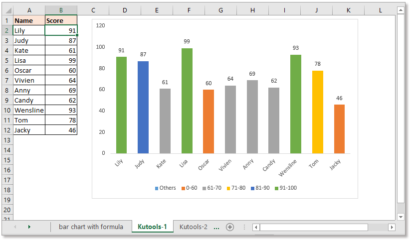
Change chart color based on value in Excel

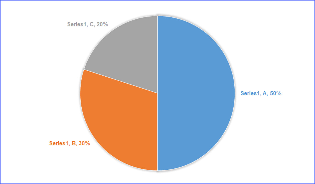
Question: labels in an Excel doughnut chart Open your Excel document and click on your chart. In the upper bar you will find the "Diagram Tools". Click on the "Design" tab. In the "Data" group, click the "Select data" button. In the right window you will find the "Horizontal axis label". Click on "Edit". Now enter your desired names or values for the legend.

Excel Custom Chart Labels • My Online Training Hub

How to Use Cell Values for Excel Chart Labels - How-To Geek Select the chart, choose the "Chart Elements" option, click the "Data Labels" arrow, and then "More Options." Uncheck the "Value" box and check the "Value From Cells" box. Select cells C2:C6 to use for the data label range and then click the "OK" button. The values from these cells are now used for the chart data labels.

Excel Course: Inserting Graphs

Change axis labels in a chart - support.microsoft.com Your chart uses text from its source data for these axis labels. Don't confuse the horizontal axis labels—Qtr 1, Qtr 2, Qtr 3, and Qtr 4, as shown below, with the legend labels below them—East Asia Sales 2009 and East Asia Sales 2010. Change the text of the labels. Click each cell in the worksheet that contains the label text you want to ...

How to Make Labels the Same Color as the Pies in Pie Chart - ExcelNotes

Excel Chart Data Labels-Modifying Orientation - Microsoft Community You can right click on the data label part then select Format Axis. Click on the Size & Properties tab then adjust the Text Direction or Custom Angle. Thanks, Mike Report abuse 7 people found this reply helpful · Was this reply helpful? Yes No

Multiple Series in One Excel Chart - Peltier Tech Blog

How to Add Total Data Labels to the Excel Stacked Bar Chart Apr 03, 2013 · Step 4: Right click your new line chart and select “Add Data Labels” Step 5: Right click your new data labels and format them so that their label position is “Above”; also make the labels bold and increase the font size. Step 6: Right click the line, select “Format Data Series”; in the Line Color menu, select “No line”

Enable or Disable Excel Data Labels at the click of a button - How To - PakAccountants.com

Create Dynamic Chart Data Labels with Slicers - Excel Campus Feb 09, 2016 · Typically a chart will display data labels based on the underlying source data for the chart. In Excel 2013 a new feature called “Value from Cells” was introduced. This feature allows us to specify the a range that we want to use for the labels. Since our data labels will change between a currency ($) and percentage (%) formats, we need a ...

Shorten Y Axis Labels On A Chart - How To Excel At Excel

How to change Layout and Chart Style in Excel Follow the steps below to change the Chart Type in Excel: Select the Chart, then click the Change Chart Type button in the Type group on the Chart Design tab. A Change Chart Type dialog box will open.

E-xcel Tuts: Add Data Labels to Excel Charts

How to change Axis labels in Excel Chart - A Complete Guide Right-click the horizontal axis (X) in the chart you want to change. In the context menu that appears, click on Select Data…. A Select Data Source dialog opens. In the area under the Horizontal (Category) Axis Labels box, click the Edit command button. Enter the labels you want to use in the Axis label range box, separated by commas.

How-to Use Data Labels from a Range in an Excel Chart - Excel Dashboard Templates

Add or remove data labels in a chart - support.microsoft.com Click the data series or chart. To label one data point, after clicking the series, click that data point. In the upper right corner, next to the chart, click Add Chart Element > Data Labels. To change the location, click the arrow, and choose an option. If you want to show your data label inside a text bubble shape, click Data Callout.